Quantifying Player Performance in Buildup Play with Expected Threat
Introducing a concept called Expected Threat (xT) to model team behavior during buildup play in football

Introduction
In the blog post I will discuss here, the author, Karun Singh, introduces a new concept called Expected Threat (xT) to model team behavior during buildup play in football. The author argues that while quantitative analysis is great, we can amplify the gains of such analysis by being more adventurous with presentation, which is why his post contains a lot of interactivity. To motivate the rest of the post, the author provides an example of Arsenal’s opening goal in a game against Burnley and asks the reader to consider where the credit for the goal should be given. While the assist for the goal is given to Kolašinac on paper, Özil’s contribution is not captured in a proportional manner.
The author argues that breaking down buildup play and assigning credit to individual actors is a hard problem. This is where xT comes in. xT is a framework that models team behavior during buildup play in order to gain a deeper understanding of it. The framework is built on three main components: Event Probability, Pitch Control, and Threat.
Existing approaches
The problem of assigning credit to individual actors in a buildup play is not a new one, and there are several existing quantitative frameworks that can be used to approach this problem. However, each of these frameworks has limitations that make it difficult to accurately capture the contribution of each player. For instance, looking only at assists would not capture contributions such as Mesut Özil’s in the Arsenal-Burnley game.
On the other hand, xGChain and xGBuildup divide up the xG equally among all players involved in the play, regardless of their actual contribution. The difference in xG induced by each action in the buildup is a better approach, but it does not always capture the true threat of a pass, since a threatening pass may not always lead to a good shooting position. In the case of Özil’s pass to Kolašinac, it split the defense open, but Kolašinac did not receive it in a particularly good shooting position. Therefore, there is a need for a new framework that can accurately capture the contribution of each player in a buildup play.
What would be a better approach?
The author proposes a framework that rewards individual player actions, operates on event-level data, is independent of the end outcome of the possession, and recognizes “threatening” positions that can lead to high-xG shooting positions with high likelihood.
To reward individual player actions, the proposed model assigns a score to each player action based on how much it contributed to the build-up play. To operate on event-level data, the author uses a list of sequential events along with basic attributes for each event, such as the player in possession, time elapsed in the match, start location, end location, etc.
To be independent of the end outcome of the possession, the proposed model assigns a score to each action in isolation, disregarding what happened before and after it in the possession. The author proposes to assign a value to every location on the pitch and use the “difference in xG” approach to assign a score based on just the start and end locations of the action. Specifically, the score for the action can be the value at the end location minus the value at the start location.
To recognize “threatening” positions, the author proposes to look beyond xG and recognize high-threat locations that can lead to high-xG shooting positions. While assigning values to locations, the author considers the possibility of stringing together multiple actions to recognize high-threat locations.
To assign a threat value to every location on the pitch, the author proposes to create a “value surface” by assigning a value to every location on the pitch. This idea of assigning a value to every location on the pitch is not new, and there is a physics analogy with electric potential fields to think about.
Overall, the proposed framework addresses the deficiencies of existing approaches and provides a way to assign a threat value to every location on the pitch based on event-level data.
When in possession…
The article introduces a simplified model of buildup play in football, where a team in possession can either shoot or move the ball to a different location via a pass or a dribble until they either lose possession or score a goal. The author then uses data from the 2017–2018 season of Premier League games to analyze the behavior of players in different zones of the pitch. By examining the aggregated data, the author identifies certain attributes associated with each zone, including the move probability, shoot probability, move transition matrix, and goal probability.
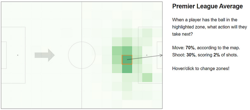
The move probability, denoted as m_x,y, is the probability that a player in possession in zone (x,y) will opt to move (i.e., pass or dribble) the ball as their next action. The shoot probability, denoted as s_x,y, is the probability that a player in possession in zone (x,y) will opt to shoot as their next action. By definition, m_x,y+s_x,y=100%.
The author also introduces the move transition matrix, T_x,y, which shows the probability that a player who moves from zone (x,y) will move to each of the other zones. The visualization provided in the article shows these probabilities in shades of green.
Finally, the author introduces the goal probability, denoted as g_x,y, which is the probability that a player who shoots from zone (x,y) will score a goal. The author notes that this quantity is essentially a simple implementation of expected goals (xG).
The author notes that their simplified model can be thought of as a Markov model, where each grid location is a state and passing or dribbling leads to state transitions. The author also acknowledges that their model considers only successful moves, but note that it could be extended to include attempted moves as well, at the cost of making the model more complex.
If you want to know more about Markov models applied in football analytics visit the link below:
Assessing Individual Offensive Contributions and Tactical Strategies in Soccer with Markov Chains
Using Markov chains to understand the value of game situations and quantifying player’s contribution to creating…medium.com
Looking beyond checkmate
In this section of the blog post, the author discusses the limitations of purely shot-based models like expected goals (xG) when analyzing buildup play. The problem with such models is that they do not account for meaningful actions that lead to good shooting positions multiple actions later. The author quotes Cervone et al., who state that such models are akin to analyzing a chess match based only on the move that resulted in checkmate, leaving unexplored the possibility that the key move occurred several turns before. Thus, the author proposes a solution to assign values to zones that reflect not just their immediate shooting value but also the future rewards they can bring through movements of the ball to other zones. The key intuition here is that when a team has possession in a particular zone, they have a choice: they can either shoot and score with some probability or move the ball to a different location. Given this background, the author formulates the problem as a mathematical optimization problem, which is discussed in the subsequent sections of the blog post.
Deriving xT
Here it is discussed how to derive the Expected Threat (xT) metric for football, which values the locations on the pitch based on the potential danger they pose to the opponent. The author works with a 16x12 grid on the pitch, which gives 192 zones, and he defines V_x,y as the value assigned to zone (x,y) by their algorithm.
When the ball is at zone (x,y), the player has two options: shoot or move the ball. If the player shoots, the expected payoff is g_x,y, which is the probability of scoring from that zone based on past data. However, if the player chooses to move the ball, they have 192 possible zones to move it to, and the expected payoff is the value at the new zone, V_z,w. To compute the expected payoff for all 192 choices, the author uses the move transition matrix T_x,y, which is based on past data and indicates where the player is likely to move the ball to from zone (x,y). The payoff for moving the ball to zone (z,w) is then T_x,y→(z,w) × V_z,w, which is the probability of moving to that zone times the reward from that zone.
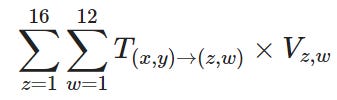
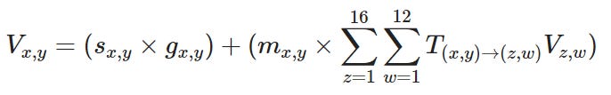
To obtain the total expected payoff for moving the ball, the author sums this quantity over all 192 possible zones. The final value for zone x,y is then obtained by weighting the payoff for shooting and the payoff for moving the ball based on their probabilities: s_x,y is the probability of shooting from zone (x,y) based on past data, and m_x,y is the probability of moving the ball. The author then defines xT as the sum of the weighted payoffs for shooting and moving the ball.
The xT metric values locations based not just on the immediate shooting threat but also on the potential to induce danger later in the possession sequence. It is inherently designed to capture a notion of “threat” and can be computed for any resolution of the pitch based on the available data. Overall, this approach provides a quantitative way to evaluate the potential threat of different locations on the football pitch, which can be useful for tactical analysis and decision-making in the game.
But wait, there’s more…
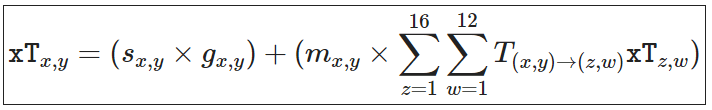
The blog post explains a workaround to overcome the cyclic dependency issue in the formula to compute xT value for a zone (x,y). The flaw in the formula is that computing xT value for a zone requires the knowledge of xT value for all other zones, forming a cyclic dependency. To break this cyclic dependency and achieve convergence, the author suggests initializing all xT values to 0 for all zones and evaluating the formula iteratively until convergence. Empirically, the author found 4–5 iterations to be sufficient for convergence, but this may vary based on the dataset.
This iterative process not only breaks the cyclic dependency but also provides interpretability to the xT values. At the first iteration, xT values represent how good a shooting position is. After the first iteration, the xT computation includes the possibility of “move, then shoot” in addition to just “shoot.” In subsequent iterations, the xT computation considers multiple moves before the checkmate, making it interpretable as the probability of scoring within the next n actions at iteration n. Thus, this approach provides a natural meaning to xT, similar to its cousin xG, and allows for better interpretability of the model.
Visualizing xT
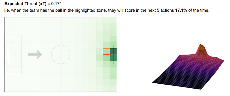
The section discusses the visualization of xT, which is the measure of the probability of scoring a goal from a particular location on the pitch within a specific number of actions. The author presents a 2D and 3D visualization of the xT value surface generated by using the events from all the matches of the 2017/18 Premier League season.
The visualization allows us to see how the xT values change over different iterations of the algorithm. As we step through the iterations, we can observe some interesting features. At iteration 0, the map is flat since we initialize xT = 0 for all zones. At iteration 1, the model is essentially computing an xG model, i.e., it values positions as though shooting was the only option, and passing and dribbling did not exist. As we move to the subsequent iterations, we can see the xT values spread to areas further away from the goal. This is because each iteration allows us to account for one more action in the buildup play. After 4–5 iterations, the xT values start to converge to a reasonable degree. Overall, the visualization provides an intuitive understanding of the xT values and how they vary across different zones on the pitch.
Applying xT
In this section of the blog post, the author discusses how to apply the xT metric to evaluate individual player actions in buildup play. The goal is to compute the difference in xT between the start and end locations of a player’s action. This difference in xT represents the value of the action, i.e., the % change in the team’s chances of scoring in the next five actions due to the action. To illustrate how this works, the author revisits the Kolašinac-Özil credit assignment problem from earlier, where Özil made a pass to Kolašinac, who then assisted a goal. The author computes the difference in xT due to each player’s action and find that Özil is responsible for 86% of the net change in xT, while Kolašinac is responsible for the remaining 14%. The author notes that, in this example, he had discretized the start and end locations to a grid cell, but for more precise analysis, one could use bilinear interpolation to compute the xT map with a fixed-size grid and then use exact location coordinates to compute more precise estimates for player actions.
Top xT creators
The xT framework has been used to identify the top creators of danger during the 2017/18 Premier League season. The table presented in the post shows the top 15 players in the league whose actions created the highest cumulative change in xT. It is interesting to note that this ranking is not based on the normalized number of actions taken but on the raw sum of xT created. This means that it highlights players who not only know how to create danger but those who do it consistently at a high volume. It is also worth noting that the inclusion of José Holebas at #3 might surprise some readers, but the left-back had established himself as Watford’s most consistent and most dangerous creator.

The top spot in the table is occupied by Kevin De Bruyne of Manchester City, with 28.033 xT created. Cesc Fàbregas of Chelsea is second, with 20.538 xT created, and José Holebas of Watford is third, with 18.487 xT created. The rest of the players in the top 15 are a mix of attacking midfielders, wingers, and central midfielders from some of the top Premier League teams.
The post also notes that the xT framework opens the door for a host of other applications beyond simple credit assignment in buildup play. The example given is computing xT on a per-team basis. This would allow for the identification of team-specific information, as different teams behave differently in possession, prioritizing different areas of the pitch and exploiting different paths to goal based on their strengths and weaknesses. This would be a particularly interesting avenue of research for coaches and analysts, who could use this information to optimize their team’s performance on the pitch.
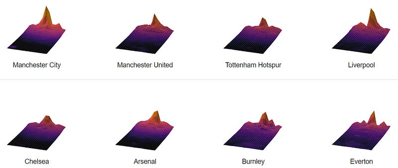
Visualizing per-team xT
In this section, the author focuses on visualizing per-team xT maps, based on data from the 2017/18 season of the Premier League. The xT maps reveal a lot of variance across different teams, with differences in the shape and height of the xT curves. The author points out that the shape of the xT curve for Manchester City and Tottenham Hotspur is similar, which means that they value the ball in similar areas of the pitch, but the xT magnitudes are very different. This implies that given the ball in the same position, Manchester City is much more threatening than Tottenham Hotspur due to their higher conversion rate of possessions into goals.
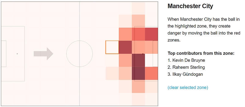
While these per-team xT maps are interesting to look at, the underlying data is powerful as it can give us a team-specific view into how danger is created through buildup play. For example, during pre-match analysis, one useful question to answer might be: where on the pitch do our opponents tend to create the most danger from? To answer this, we can use our opponent’s xT map to value all of their actions from past matches, and aggregate these values based on the start location of the action. In other words, for each grid location, we can look at the actions that originated there and sum the xT created by these actions. This will give us a per-location cumulative value that will highlight the amount of danger created from different areas of the pitch. Additionally, by highlighting the common end zones of actions starting in a particular zone, we can start to see our opponent’s most dangerous passages of play. To make this even more useful for tactical preparation, we might want to know who are the players that are responsible for creating threat through these passages.
Who creates danger from where?
The analysis of data from the 2017/18 season shows that Manchester City tends to create the maximum threat from the green zones. The per-location cumulative value is obtained by valuing all of the team’s actions from past matches and aggregating these values based on the start location of the action. This approach helps in identifying the areas of the pitch from which the team tends to create the most danger through buildup play.
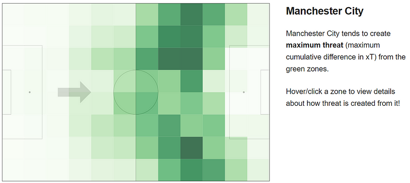
By highlighting the common end zones of actions starting in a particular zone, the most dangerous passages of play of the team can be identified. The visualization provided in the blog post can help in understanding the key players responsible for creating threat through these passages. The analysis of xT maps can be used during pre-match analysis to prepare tactics for playing against a particular team. The findings from this study can be used to develop strategies to counter Manchester City’s threat creation from the green zones.
Future work
The xT framework introduced in this blog post has a lot of potential for further exploration and application. The author suggests that the xT framework could be used to identify and analyze patterns of play, such as counter-attacks, by tracking changes in xT over the course of a possession sequence. This could provide a deeper understanding of the tactical choices made by teams during gameplay.
Furthermore, the xT framework could be applied at the player level to evaluate individual players’ decision-making relative to their team’s xT profile. By analyzing a player’s history of creating actions that lead to high xT gains, teams could assess whether a player would be a good fit for their system. This could be useful for scouting new players and making strategic decisions about team composition. Overall, the xT framework is a promising tool for understanding and analyzing football gameplay, with many exciting possibilities for future research and application.
References
Singh, K. (2019). Introducing expected threat (XT). https://karun.in/blog/expected-threat.html