Why Your xG Model Might Be Wrong: The Bayesian Solution to Accurate Scoring Predictions
Using Bayesian Hierarchical Methods to Correct Player and Position Factors in Expected Goals Predictions.
1 Introduction
The concept of expected goals (xG) has become a fundamental metric in football analytics, estimating the likelihood of a shot resulting in a goal based on contextual features such as shot distance, angle, and body part used. However, mainstream xG models do not account for player-specific attributes, leading to a uniform probability assignment for identical shots taken by different players. This limitation disregards variations in individual skill levels, exemplified by a scenario where Lionel Messi and a National League player take the same shot under identical conditions but are assigned the same xG value. Intuitively, Messi's superior finishing ability should yield a higher probability of scoring, yet conventional xG models fail to incorporate this effect.
This study seeks to determine whether player and positional effects influence xG predictions by employing Bayesian hierarchical modelling. The methodology introduces hierarchical structures based on player identity or playing position, allowing for individual or positional adjustments to goal probabilities. To validate this approach, the results from hierarchical Bayesian models will be compared against a traditional frequentist xG model, establishing a baseline for group-independent predictions. Subsequently, the hierarchical models will be evaluated against non-hierarchical Bayesian models to assess the impact of incorporating player- and position-based hierarchies. If player skill or positional influence significantly affects goal probability, hierarchical models should diverge from non-hierarchical counterparts, reinforcing the hypothesis that xG should incorporate player-specific effects.
2 Related Works
Despite the increasing availability of football data, skepticism remains about its effectiveness in improving performance due to the sport's complexity. However, advancements in data collection and tracking technologies have enabled analytics to influence performance evaluation, scouting, and injury risk assessment. While many clubs keep their data-driven strategies private, publicly available research has shown the value of football analytics. Traditional metrics like possession percentages have evolved into advanced models, such as real-time goal probability assessments based on expected goals (xG).
xG has been instrumental in football analytics, providing insights beyond match outcomes by estimating scoring probabilities. This metric helps mitigate biases from chance-influenced results, offering a more objective measure of performance. Over time, various xG models have incorporated machine learning techniques, integrating contextual factors like defensive pressure, speed of play, and spatial positioning to enhance predictive accuracy.
Some studies have explored the impact of individual player attributes on xG, incorporating qualitative adjustments to improve predictions for specific players and positions. Positional effects have also been analyzed, revealing systematic differences in xG adjustments across roles. Player-specific models have demonstrated that exceptional individuals can significantly outperform standard xG expectations.
While most xG models have relied on frequentist methods, Bayesian approaches have been applied in related areas of football analytics, such as match outcome predictions and team performance assessments. Bayesian hierarchical models, which account for multi-level group effects, remain underutilized in xG estimation. These models offer a structured way to incorporate player and positional effects, particularly when data is sparse, enabling a more refined assessment of shooting ability and goal-scoring efficiency.
By framing xG estimation within a hierarchical Bayesian framework, individual finishing ability can be quantified more precisely, aiding scouting and player evaluation. This approach enhances the predictive accuracy of xG by formally integrating player and position information into a probabilistic model.
3 Methodology
3.1 Preliminaries on xG Calculation
Traditional xG models are commonly built using a frequentist framework, with logistic regression being a natural choice for modeling goal probabilities.
Logistic regression maps a set of independent variables to a binary dependent outcome, transforming the linear combination of predictors into probability values. The frequentist approach used in this paper begins by developing a baseline xG model with a minimal set of predictors before incrementally introducing additional shot features to improve predictive performance. The objective is to establish a baseline xG model comparable to industry-standard models such as StatsBomb’s proprietary xG model.
3.2 On the Bayesian Predictive Modelling of xG Models
A Bayesian predictive framework extends xG modeling by incorporating uncertainty quantification and prior knowledge. The posterior predictive distribution provides a probabilistic estimate of future goal-scoring probabilities, given observed data and inferred model parameters
Bayesian inference updates prior beliefs about model parameters based on the observed data, resulting in posterior distributions that provide a full range of plausible parameter values rather than point estimates. Sampling from the posterior predictive distribution allows for uncertainty quantification, capturing both variability in observed data and parameter estimation uncertainty. This probabilistic approach contrasts with frequentist methods, which assume fixed parameter values.
3.3 Bayesian Logistic Regression
Bayesian logistic regression extends the frequentist logistic regression model by treating its parameters as random variables with associated probability distributions. Rather than obtaining fixed point estimates, Bayesian logistic regression produces posterior distributions for model parameters, enabling uncertainty quantification.
The model follows the Bernoulli likelihood:
where Yi represents the binary goal outcome (1 if goal, 0 otherwise), and pi is the probability of scoring.
The Bayesian logistic model incorporates prior distributions for coefficients βj, which are updated using observed data to form the posterior distribution. The inference process relies on computational methods such as Markov Chain Monte Carlo (MCMC) sampling and variational inference.
To evaluate group-level effects, the paper introduces hierarchical Bayesian models.
3.4 Data
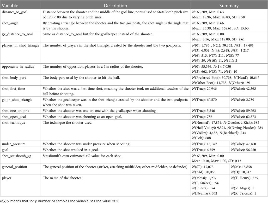
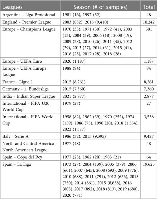
The dataset used in this study consists of 63,309 open-play shots from StatsBomb’s publicly available event data, extracted using the StatsBombPy Python package. The data spans multiple leagues and seasons, with 42 features per shot, including location, shot characteristics, and contextual information.
Key engineered features include:
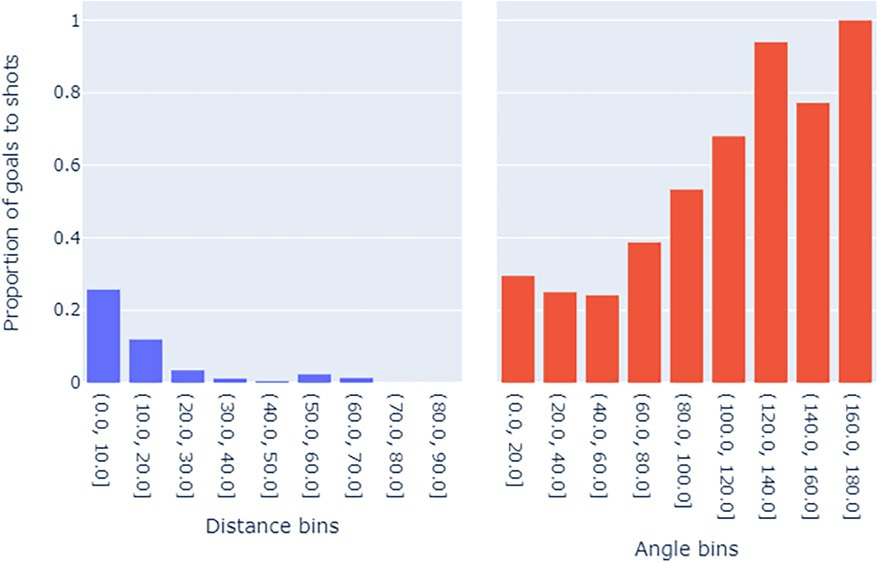
Distance to Goal: Calculated as the Euclidean distance from the shot location to the goal center.
Shot Angle: Computed using the cosine rule to determine the angle between the shooter and goalposts.
Freeze Frame Features: Includes goalkeeper’s position relative to the shot, number of players in the shot triangle, and the number of opponents within a 1m radius of the shooter.
Positional Grouping: Players are categorized into four groups—Strikers (ST), Attacking Midfielders (AM), Midfielders (M), and Defenders (D)—based on their primary position.
Body Part Used: The preferred foot for each player is inferred from passing data, differentiating shots taken with the dominant foot from those taken with the weaker foot.
3.5 Reference Models
To establish a basis for evaluating Bayesian hierarchical models, two frequentist xG models are defined:
StatsBomb xG Model: A proprietary benchmark model used for comparison, though its methodology is undisclosed.
Baseline xG Model: A logistic regression model incorporating shot distance, angle, and their interaction as predictors
Extended xG Model: Incorporates additional shot features such as goalkeeper position, number of defenders, shot technique, and contextual pressure to improve predictive accuracy.
3.6 Bayesian xG Models
Bayesian hierarchical modeling is employed to account for player- and position-based variations in xG estimation. Three versions of Bayesian hierarchical xG models are defined:
Bayes-xG1: A baseline hierarchical model grouping shots by position.
Bayes-xG2: An extended hierarchical model incorporating additional shot features while grouping by position.
Bayes-xG3: A hierarchical model grouping shots by individual players.
3.6.2 Choice of Priors
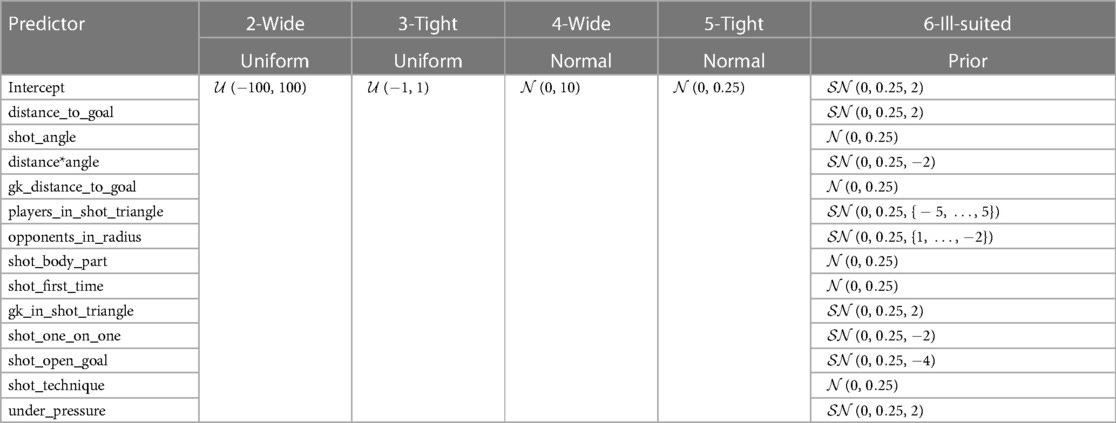
A critical aspect of Bayesian modeling is the selection of prior distributions. The priors for predictor coefficients are assigned based on prior knowledge of their expected effects:
Distance to Goal: μ=−1, α=−1 (negative effect on goal probability).
Shot Angle: μ=1, α=1 (positive effect on goal probability).
Players in Shot Triangle: α={5,…,−5} (more players decrease goal probability).
Goalkeeper Presence in Triangle: α=−2 (reduces scoring probability).
Open Goal: α=4 (significantly increases scoring probability).
General Position: α={ST: 2, AM: 1, M: 0, D: -2} (strikers have highest expected goal probability).
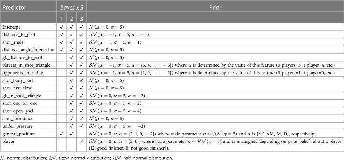
A standard prior standard deviation of σ=5 is used to balance informativeness and flexibility.
3.7 Model Development
The computational implementation of Bayesian models is performed in Python 3.8+ using the bambi package, a framework for fitting Bayesian generalized linear multilevel models. Logistic regression models are implemented using sklearn, while Bayesian inference relies on Markov Chain Monte Carlo (MCMC) sampling. The models are trained with:
1,500 posterior draws per chain (4 chains, 6,000 total samples).
A burn-in period of 250 draws.
Target acceptance ratio of 95%.
Bernoulli likelihood function for binary goal outcomes.
To mitigate dataset imbalance, the analysis is restricted to a single league to ensure diversity in player matchups, reducing bias from over-representation of specific teams.
4 Experimental Analysis
The experimental evaluation of the proposed Bayesian hierarchical xG models is structured into six key analyses:
Comparison of frequentist xG models to the benchmark StatsBomb model.
Positional adjustments to xG using Bayesian hierarchical modeling.
Player-specific adjustments to xG using Bayesian hierarchical modeling.
Validation of Bayesian models across multiple leagues.
Sensitivity analysis of prior selection on Bayesian xG predictions.
Quantification of uncertainty using posterior predictive analysis.
4.1 Frequentist xG Models
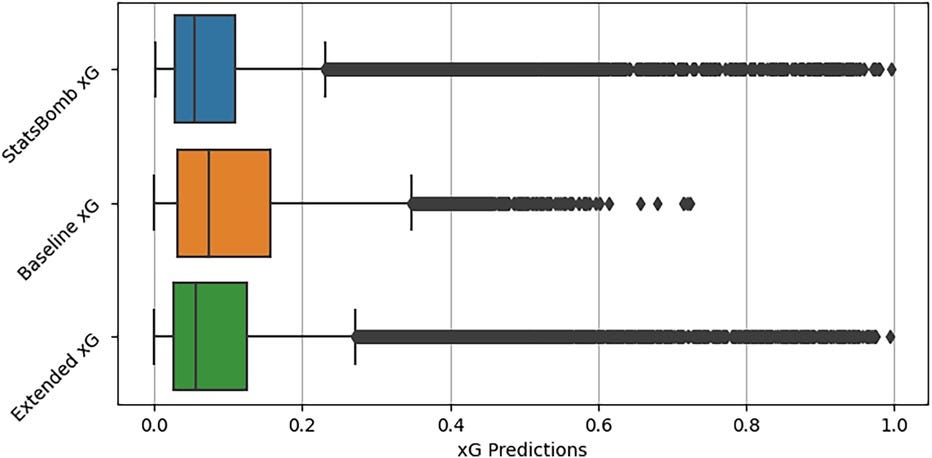
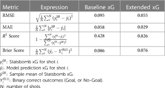
The first set of experiments evaluates the performance of frequentist logistic regression models (Baseline xG and Extended xG) on the full dataset of 63,309 shots, comparing their predictions to the StatsBomb benchmark xG model. The xG distributions of these models are visualized, revealing that the Extended model aligns more closely with StatsBomb’s xG values than the Baseline model. The extended model, incorporating additional shot features, exhibits lower variance and more extreme predicted values, reflecting improved goal probability estimation.
Model performance is assessed using R², mean absolute error (MAE), and root mean square error (RMSE). The Extended model significantly outperforms the Baseline model, achieving a Brier score close to StatsBomb’s 0.075, indicating near-parity with an industry-leading xG model.
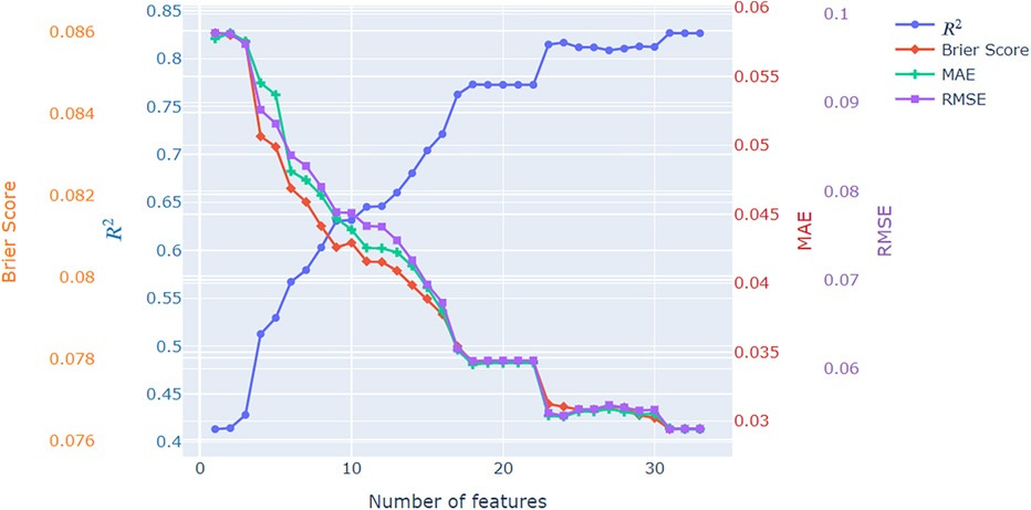
A feature ablation study further illustrates the impact of additional predictors on model performance, demonstrating significant gains in predictive accuracy with the inclusion of engineered variables such as goalkeeper positioning and defensive pressure.
4.2 Positional Analysis via Bayesian Models
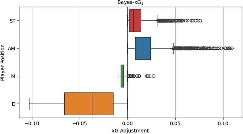
The second experiment investigates the effect of player positions on xG by introducing hierarchical Bayesian models. The Baseline and Extended xG models are re-estimated with position-level grouping effects, yielding Bayes-xG1(Baseline + positional hierarchy) and Bayes-xG2 (Extended + positional hierarchy).
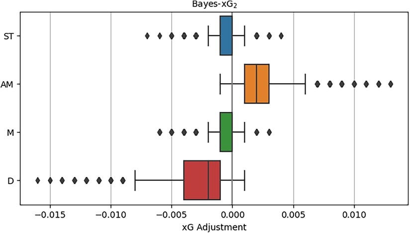
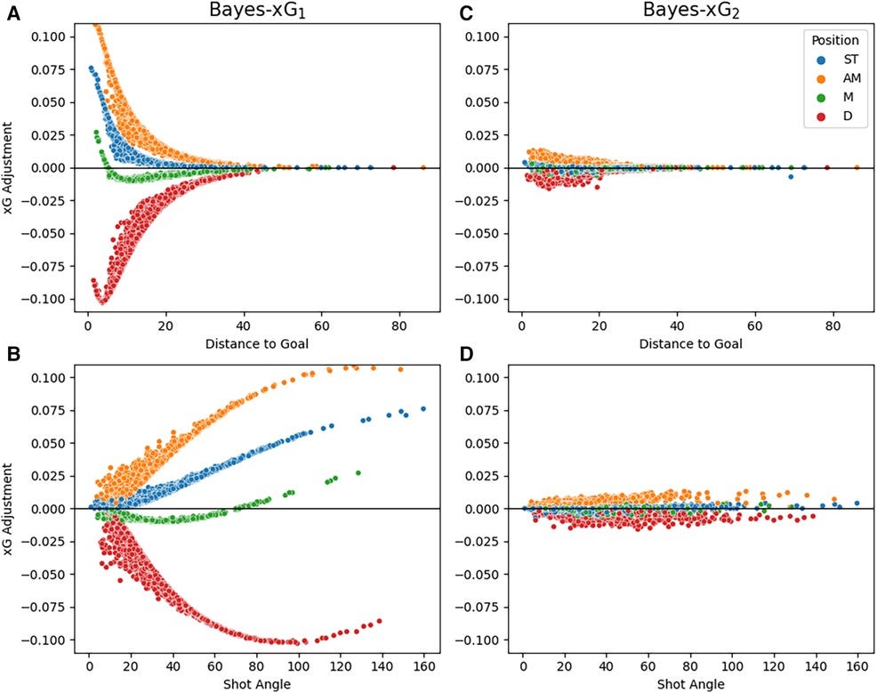
Comparison of single-level and hierarchical models reveals systematic positional adjustments to xG predictions. Defenders receive substantial negative xG adjustments, midfielders exhibit minor adjustments, while strikers and attacking midfielders receive positive corrections. Surprisingly, attacking midfielders show higher positive xG adjustments than strikers, suggesting superior shot conversion ability in high-xG scenarios.
To validate these findings, a theoretical adjustment using Bayes’ Theorem is computed and compared to hierarchical model estimates, revealing strong alignment between theoretical and empirical adjustments.

The introduction of additional predictors in Bayes-xG2 significantly reduces the magnitude of positional adjustments, suggesting that positional effects are largely accounted for by shot-specific features rather than intrinsic positional differences.
Further analysis across shot distance and angle reveals that defenders exhibit the largest negative xG corrections at extreme shot distances, while attacking midfielders maintain the highest positive adjustments at close-range shots. However, in the Extended model (Bayes-xG2), these distinctions nearly vanish, reinforcing the hypothesis that shot context, rather than position alone, determines xG.
4.3 Player-Specific Analysis via Bayesian Models
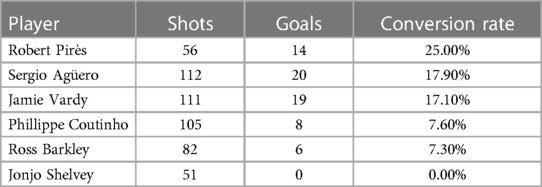
The third experiment extends hierarchical Bayesian modeling to player-level adjustments. The Bayes-xG3 model groups data by individual players rather than positions, allowing for player-specific corrections. Due to computational constraints, only a subset of players is analyzed, selected based on conversion rates. High-performing goal scorers (e.g., R. Pirès, S. Agüero, J. Vardy) are expected to receive positive xG corrections, while inefficient shooters (e.g., J. Shelvey) should receive negative adjustments.
Results reveal significant player effects on xG. R. Pirès exhibits the highest positive xG corrections, with some adjustments exceeding 0.3 above baseline xG, reflecting his ability to convert low-xG opportunities. Conversely, Shelvey receives strong negative xG corrections, indicating poor shot conversion despite frequently taking high-xG chances.
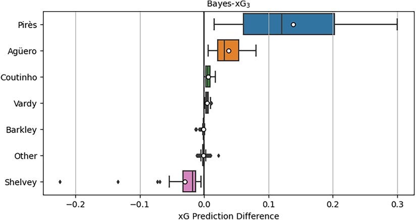
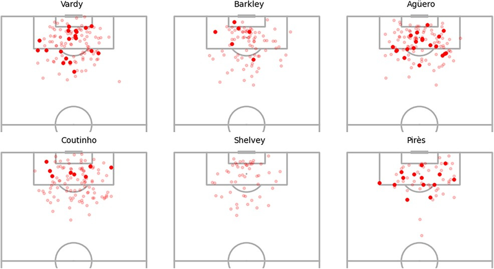
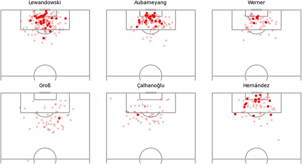
Visualization of shot maps supports these findings: high-adjustment players (e.g., Pirès, Agüero) consistently score from difficult positions, while low-adjustment players (e.g., Shelvey) fail to convert central, high-xG opportunities.
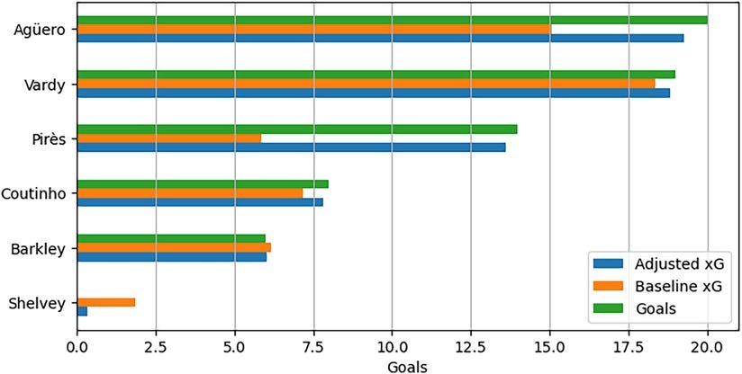
Aggregated xG comparisons further validate the model, with adjusted xG estimates aligning more closely with actual goals scored than the baseline xG model.
4.4 Validation Across Multiple Leagues
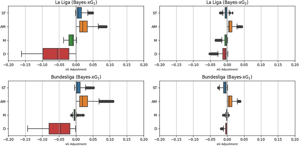
To generalize findings beyond the English Premier League, the Bayesian hierarchical models are applied to La Liga(19,000 shots) and Bundesliga (7,500 shots). Results confirm the consistency of positional effects across leagues: defenders exhibit negative xG corrections, attacking midfielders receive positive adjustments, and positional adjustments shrink in the extended model (Bayes-xG2).
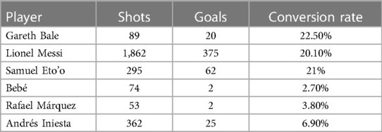
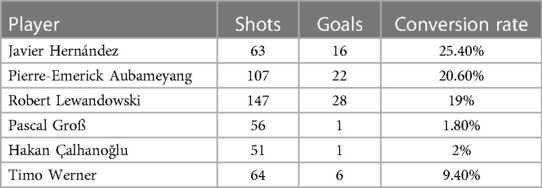
Player-specific corrections in Bayes-xG3 are validated using high- and low-conversion players from La Liga (e.g., G. Bale, L. Messi) and Bundesliga (e.g., P. Aubameyang, H. Çalhanoğlu). As expected, Messi and Bale receive strong positive xG corrections, while underperforming shooters receive negative adjustments. Notably, Aubameyang, despite a high conversion rate, exhibits negative adjustments, indicating that his goals come primarily from high-xG chances.

4.5 Impact of Prior Selection
Sensitivity analysis examines the influence of prior distributions on Bayesian xG predictions. The extended single-level Bayesian model is re-estimated with six different prior configurations, including uniform, normal, and ill-suited priors.
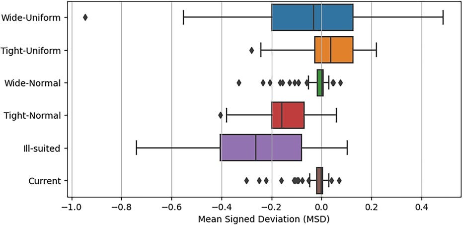
Comparisons reveal that wide uniform priors produce erratic xG estimates, while tight normal priors systematically underestimate goal probabilities. The best performance is achieved with wide normal priors, which closely match the benchmark model.
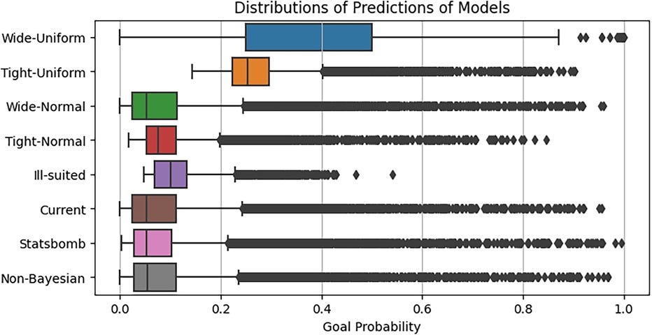
Mean signed deviation (MSD) analysis quantifies the deviation of each prior’s predictions from the non-Bayesian extended model. Wide normal priors exhibit the smallest MSD values, while tight normal and ill-suited priors show strong over- or under-prediction tendencies. These results highlight the importance of selecting well-informed priors that balance informativeness with flexibility.
4.6 Uncertainty Quantification
The final experimental case examines the uncertainty inherent in Bayesian xG predictions using posterior predictive densities. For each position in Bayes-xG1 and Bayes-xG2, posterior distributions are analyzed for a representative shot with StatsBomb xG ≈ 0.15. Results reveal that Bayes-xG2 consistently exhibits higher uncertainty than Bayes-xG1, with wider 95% high-density intervals (HDI) reflecting greater variance in xG estimates. This increased uncertainty is attributed to the richer feature set of Bayes-xG2, which captures more nuanced shot dynamics.
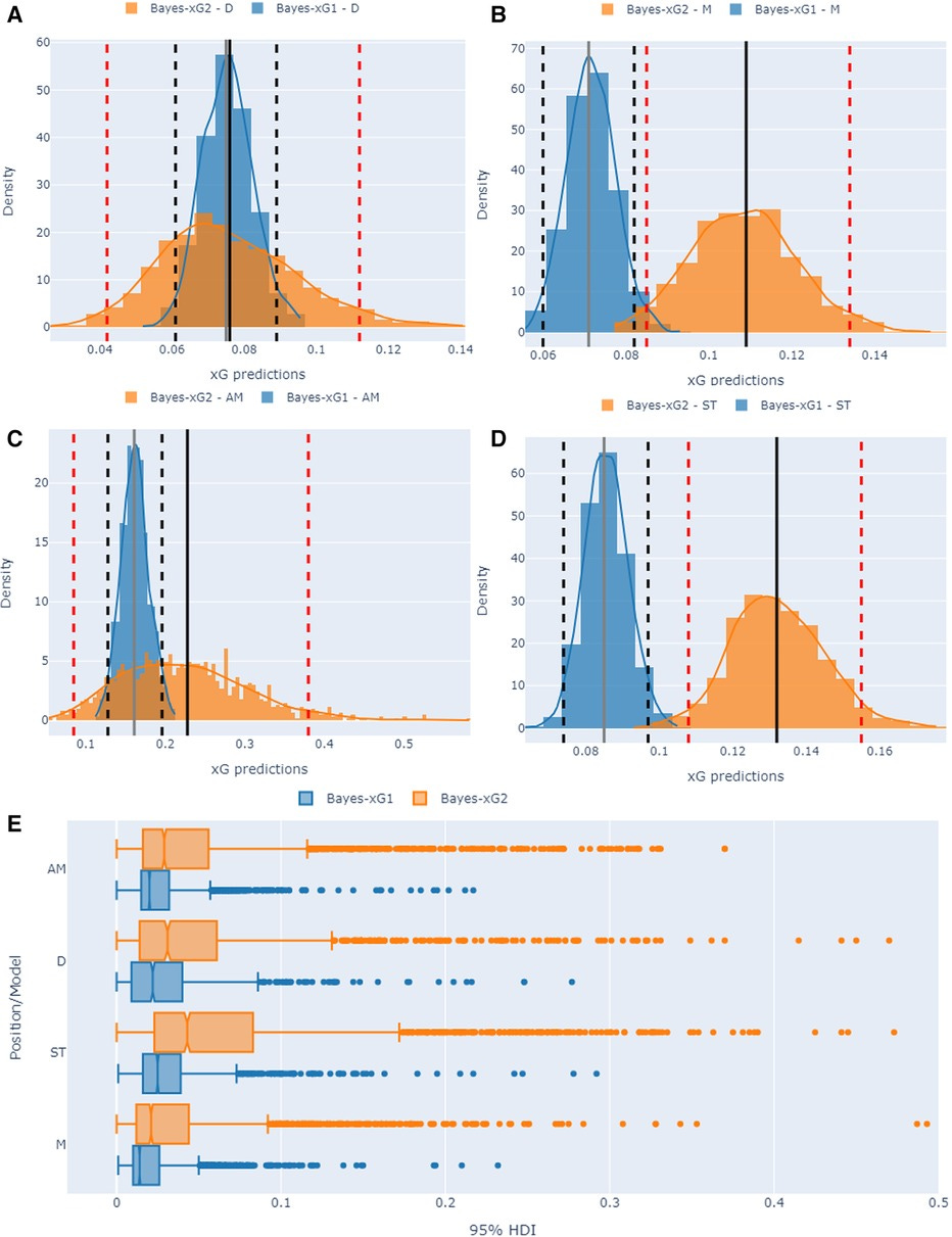
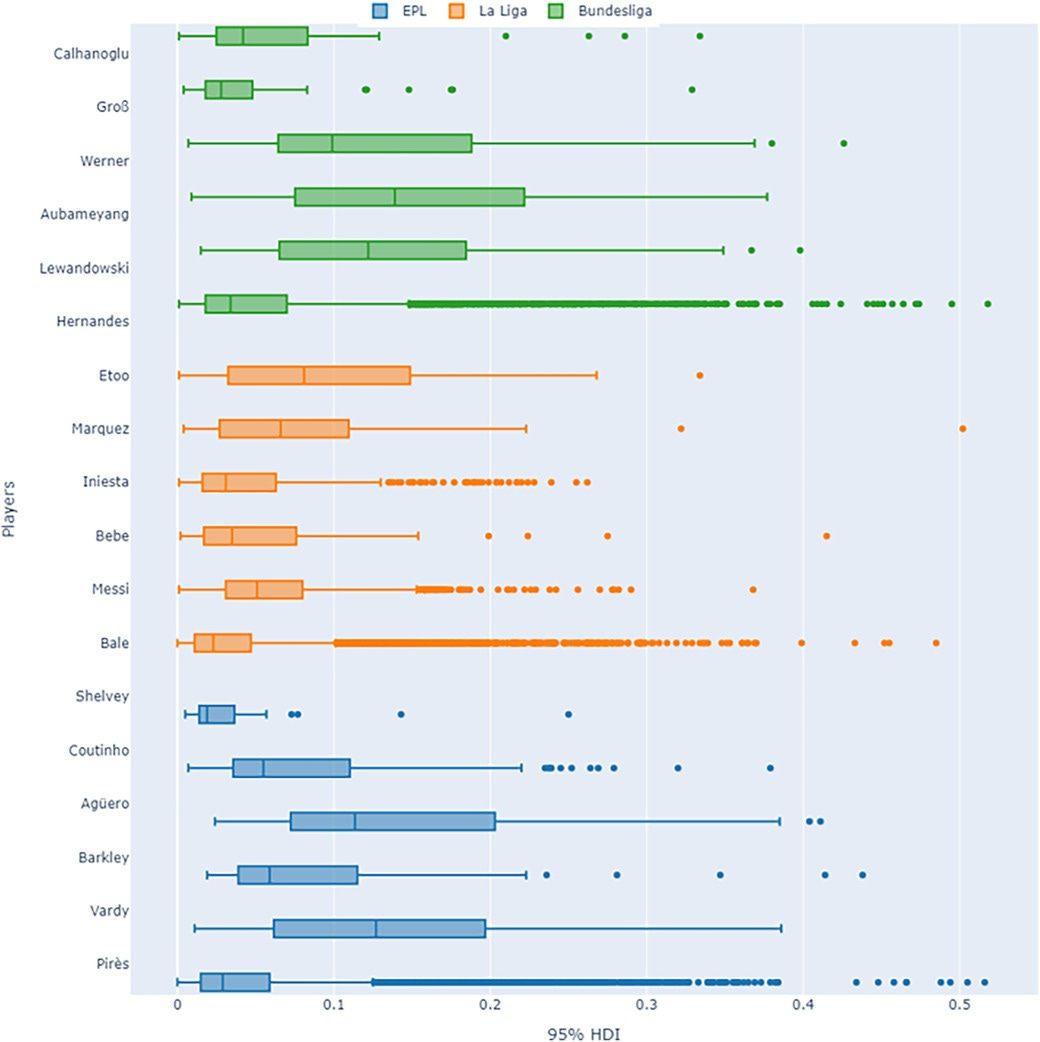
A similar analysis for Bayes-xG3 reveals that high-adjustment players (e.g., Pirès, Bale) exhibit significantly wider HDI values than average players, indicating greater variability in their shot probabilities. The model’s ability to capture player-specific uncertainty is particularly valuable for scouting and player evaluation, allowing for a probabilistic assessment of finishing ability.
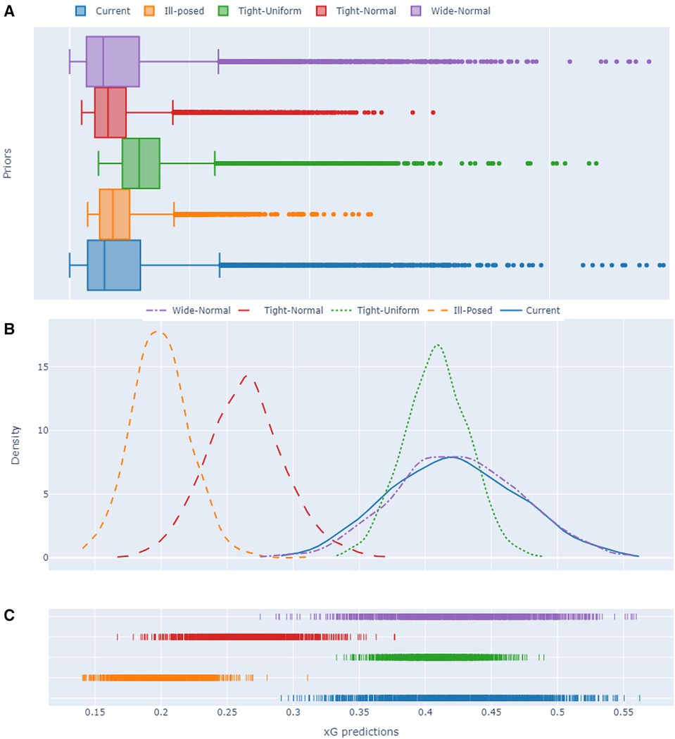
Finally, posterior predictive distributions are analyzed under different prior configurations. Wide normal priors yield the highest uncertainty, while tight priors produce overconfident, biased predictions. The chosen priors provide a balance between prediction accuracy and uncertainty quantification, ensuring robust inference.
5 Final remarks & conclusion
This study challenges the assumption that all players have identical shot conversion probabilities, demonstrating the necessity of player-specific adjustments in expected goals (xG) modeling. Bayesian hierarchical models revealed that while positional effects on xG disappear when controlling for shot-specific conditions, player-specific effects persist. Strikers and attacking midfielders initially showed positive xG adjustments, while defenders had negative corrections, but these positional trends diminished in more advanced models. However, individual players like Pirès, Bale, and Agüero consistently exceeded their expected xG, while others, such as Shelvey and Werner, underperformed, confirming distinct finishing ability variations.
The findings have key implications for scouting and player evaluation, allowing analysts to distinguish elite finishers from players reliant on high-xG opportunities. For example, Agüero’s superior finishing ability is reflected in a higher adjusted xG compared to Vardy, whose goal output closely matches his unadjusted xG due to Leicester’s counter-attacking style. Team-specific tactics influence goal-scoring opportunities, emphasizing the importance of contextual factors in player evaluation.
Uncertainty analysis highlighted the robustness of Bayesian hierarchical models, showing that well-informed priors improve model accuracy and align predictions with industry benchmarks. The approach enables a deeper understanding of finishing skill variability, particularly for high-performing players. Future research should explore team-level effects, tracking-based metrics, and dynamic xG models to enhance real-time predictive analytics.
In summary, traditional xG models fail to capture player-specific differences in finishing ability. Bayesian hierarchical modeling provides a superior framework for incorporating these effects, making it a valuable tool for scouting, tactical analysis, and advanced football analytics.
References
Scholtes, A., & Karakuş, O. (2024). Bayes-xG: player and position correction on expected goals (xG) using Bayesian hierarchical approach. Frontiers in Sports and Active Living, 6, 1348983. https://www.frontiersin.org/journals/sports-and-active-living/articles/10.3389/fspor.2024.1348983/full


